Strategies for Mall Customers (Analysis and ML)

Customer Segmentation Analysis: Uncovering Insights from Mall Customer Data

9/11/2024

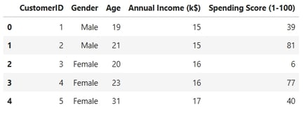
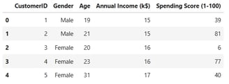
The dataset used in this analysis is sourced from Kaggle. In this project, I will perform customer segmentation to categorize mall customers into distinct groups based on key attributes such as age, annual income, and spending habits.

This type of analysis is highly valuable for mall and shop owners or managers, as it enables them to identify and target specific customer segments effectively.

Younger customers, such as kids or young adults, are more likely to spend on categories like video games, sports apparel, or fast fashion.
Older customers may prioritize spending on dining experiences, travel-related services, or similar offerings.
Spending behavior is also heavily influenced by customers' budgets, making income a critical factor in understanding purchasing patterns.

By leveraging these insights, businesses can tailor their marketing strategies, optimize product offerings, and enhance customer engagement to drive revenue growth.

Customer Segmentation Analysis: Insights from Mall Customer Data

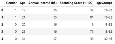
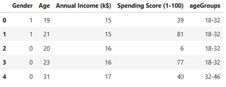
1. Data Loading, Null Value, and Duplicate Value Assessment

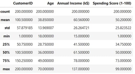
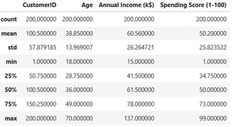
Descriptive Statistics

This step is crucial for identifying potential outliers or anomalous values in the dataset, ensuring the integrity and reliability of the analysis.

Outlier Detection

To identify potential outliers, I have generated boxplots for the numerical variables in the dataset. This visualization provides a clear and intuitive way to detect anomalies and extreme values that may impact the analysis.

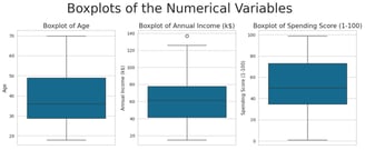
Only one outlier was identified in the dataset, and it is not significantly distant from the rest of the data. As such, it does not require any corrective action or further treatment.

2. Exploratory Data Analysis (EDA)

To better understand the underlying distributions of the numerical variables, I am calculating skewness and kurtosis. These metrics provide insights into the shape and tail behavior of the data, helping to identify deviations from normality and inform subsequent preprocessing steps.

Key Observations:

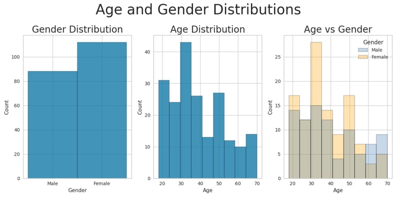
Gender Distribution:
The dataset contains a higher proportion of female customers compared to males.
Age Distribution:
- The age distribution exhibits moderate right (positive) skewness.
- The kurtosis value is less than 0, indicating a relatively flat distribution with shorter tails.
- The average age of customers is 39 years.
Gender-Specific Age Trends:
- While the average age is similar for both male and female customers, there is a notable excess of male customers above 60 years old.
- Additionally, there is a higher concentration of female customers between the ages of 30 and 35.

Preprocessing Step: Age Binning
Before analyzing the income distribution, I have grouped customers into age bins to better understand and visualize age-related trends. This step helps simplify the data and uncover patterns that may not be immediately apparent in continuous age values.

Key Insights (After Age Binning):

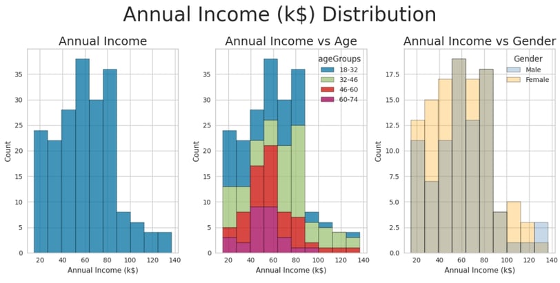
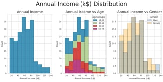
Annual Income Distribution:
- The annual income distribution exhibits moderate right (positive) skewness.
- The highest-earning group consists of customers aged between 32 and 46.
- The lowest-earning groups are customers aged 60-74 and 18-32.
High-Income Customers:
- The tail of the income distribution represents the highest-earning customers, who are likely the most valuable. The majority of these high-income customers fall within the 32-46 age range.
Gender and Income:
- There is no significant difference in earnings between male and female customers, suggesting that income distribution is relatively balanced across genders.

Age Analysis

Spending Power!!!

Key Insights:

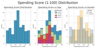
Spending Score Distribution:
- The spending score distribution is approximately bell-shaped, with near-zero skewness.
- The distribution exhibits negative kurtosis, indicating lighter tails compared to a normal distribution.
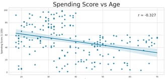
Age and Spending Score:
- On average, the spending score decreases with age.
- The 18-32 age group has the highest average spending score, while the 46-60 and 60-74 age groups have the lowest.
- A weak negative correlation exists between age and spending score (r = -0.327), further supporting this trend.
Gender and Spending Score:
- Female customers exhibit a slightly higher average spending score compared to male customers.

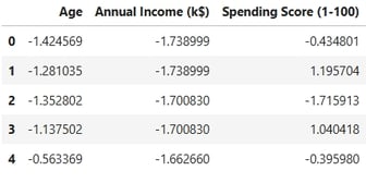
3. Data Preparation and Feature Engineering

Before training any model, whether simple or complex, it is essential to prepare and preprocess the data to ensure its suitability for modeling. This step involves transforming raw data into a format that enhances model performance and interpretability. Proper data engineering lays the foundation for robust and reliable machine learning models.

In this step, I am preparing the data for modeling by performing the following tasks:

Dropping Irrelevant Features: The CustomerID column is removed, as it does not contribute to the predictive power of the model.
Encoding Categorical Variables: The Gender variable is encoded into numerical values to make it suitable for machine learning algorithms.
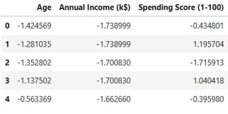
Standardizing Numerical Features: All numerical features are standardized to ensure they are on a common scale, which is critical for the performance of many machine learning models.

These steps ensure the dataset is clean, consistent, and ready for modeling.

4. KMeans Clustering

K-Means Clustering is the first clustering method I will apply to explore and analyze the data. As an unsupervised learning algorithm, K-Means groups data points into clusters based on their similarity, making it a powerful tool for identifying patterns and structures within the dataset. This approach will help uncover meaningful customer segments that can inform targeted strategies and decision-making.

Determining the Optimal Number of Clusters

To identify the most appropriate number of clusters for the K-Means algorithm, I will begin by applying the Elbow Method. This technique involves plotting the within-cluster sum of squares (WCSS) against the number of clusters and selecting the "elbow point"—the point where the rate of decrease in WCSS slows significantly. This approach provides a data-driven way to balance model complexity and clustering effectiveness.

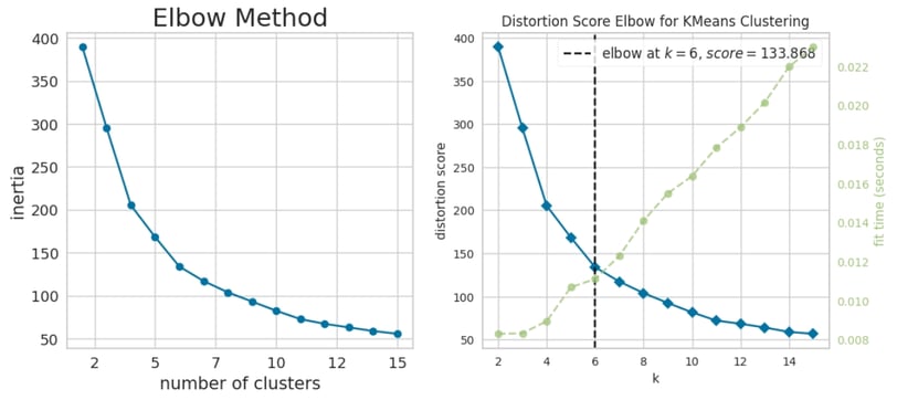
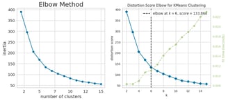
Elbow Method Analysis

Based on the Elbow Method, the optimal number of clusters appears to be k = 6, as this is the point where the rate of decrease in the within-cluster sum of squares (WCSS) begins to slow significantly.

To further validate this choice, I will also evaluate the Davies-Bouldin Score, a metric that measures the average similarity ratio of within-cluster scatter to between-cluster separation. A lower Davies-Bouldin Score indicates better-defined clusters, providing additional insight into the quality of the clustering solution.

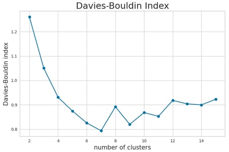
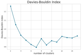
Davies-Bouldin Score Analysis

The Davies-Bouldin Score analysis suggests that a similar number of clusters (k = 6) or potentially k = 10 could be optimal, as these values yield a lower score, indicating better-defined clusters.

To further refine our choice, I will also examine the Silhouette Score, which measures how similar an object is to its own cluster compared to other clusters. A higher Silhouette Score indicates better separation and cohesion of clusters, providing additional validation for the selected number of clusters.

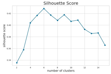
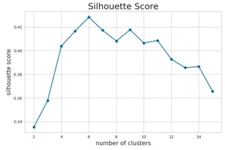
Silhouette Score Analysis

Based on the Silhouette Score analysis, k = 6 emerges as a strong candidate for the optimal number of clusters, as it demonstrates good separation and cohesion. Additionally, values of k = 9 and k = 10 also yield acceptable results, indicating that these configurations could provide meaningful clustering solutions as well.

This analysis, combined with the earlier findings from the Elbow Method and Davies-Bouldin Score, suggests that k = 6 is a robust choice, while k = 9 and k = 10 remain viable alternatives depending on the desired granularity of the segmentation.

Tuning the K-Means Model and Evaluating Results

To determine the most suitable value of k, I will evaluate clustering solutions with k ranging from 3 to 6. For each configuration, I will analyze the average values of the variables within each cluster and examine their spatial distribution. Given the relatively small size of the dataset (200 data points), I have opted to avoid higher values of k to prevent overfitting and ensure meaningful, interpretable clusters.

This approach balances granularity and practicality, allowing for a thorough exploration of the data while maintaining clarity in the resulting segmentation.

Cluster Distribution Analysis

Below, I present the cluster distributions for various values of k, beginning with the k = 3 case. This initial configuration provides a high-level overview of the data segmentation, allowing us to observe broad patterns and trends before exploring more granular clustering solutions.

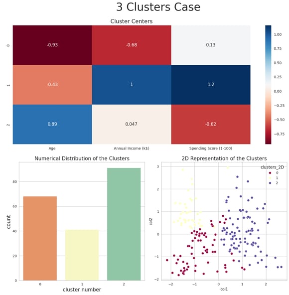
Cluster Interpretation for k = 3:

The three clusters can be characterized as follows:

Cluster 0:
- Demographic: Younger customers.
- Income Level: Low income.
- Spending Behavior: Average spending score.
Cluster 1:
- Demographic: Young to middle-aged customers (approximately 30-40 years old).
- Income Level: High income.
- Spending Behavior: High spending score.
Cluster 2:
- Demographic: Older customers.
- Income Level: Average income.
- Spending Behavior: Low spending score.

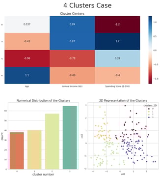
Cluster Interpretation for k = 4:

The four clusters can be characterized as follows:

Cluster 0:
- Demographic: Middle-aged customers (35-45 years old).
- Income Level: High income.
- Spending Behavior: Very low spending score.
Cluster 1:
- Demographic: Young to middle-aged customers (30-35 years old).
- Income Level: High income.
- Spending Behavior: Very high spending score.
Cluster 2:
- Demographic: Younger customers.
- Income Level: Low income.
- Spending Behavior: Medium-high spending score.
Cluster 3:
- Demographic: Older customers.
- Income Level: Medium-low income.
- Spending Behavior: Medium-low spending score.

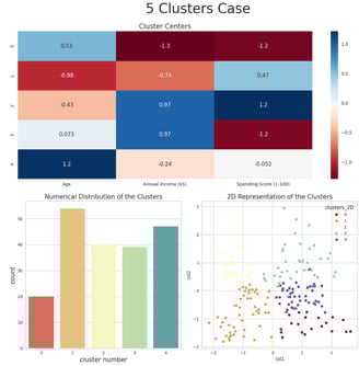
Cluster Interpretation for k = 5:

The five clusters can be characterized as follows:

Cluster 0:
- Demographic: Older customers.
- Income Level: Average income.
- Spending Behavior: Average spending score.
Cluster 1:
- Demographic: Young customers (around 30 years old).
- Income Level: High income.
- Spending Behavior: Very high spending score.
Cluster 2:
- Demographic: Younger customers.
- Income Level: Low income.
- Spending Behavior: Medium-high spending score.
Cluster 3:
- Demographic: Middle-aged to older customers (50-60 years old).
- Income Level: Very low income.
- Spending Behavior: Very low spending score.
Cluster 4:
- Demographic: Middle-aged customers (around 40 years old).
- Income Level: High income.
- Spending Behavior: Very low spending score.

These clusters offer a detailed segmentation of customers, revealing distinct patterns in age, income, and spending behavior. This granularity enables more precise targeting and personalized marketing strategies.

Cluster Interpretation for k = 6:

The six clusters can be characterized as follows:

Cluster 0:
- Demographic: Younger customers.
- Income Level: Very low income.
- Spending Behavior: Very high spending score.
Cluster 1:
- Demographic: Older customers.
- Income Level: Average income.
- Spending Behavior: Average spending score.
Cluster 2:
- Demographic: Middle-aged customers (40-45 years old).
- Income Level: Very high income.
- Spending Behavior: Very low spending score.
Cluster 3:
- Demographic: Younger customers.
- Income Level: Average income.
- Spending Behavior: Average spending score.
Cluster 4:
- Demographic: Young to middle-aged customers (30-35 years old).
- Income Level: High income.
- Spending Behavior: Very high spending score.
Cluster 5:
- Demographic: Middle-aged to older customers (50-55 years old).
- Income Level: Very low income.
- Spending Behavior: Very low spending score.

These clusters provide a highly detailed segmentation of customers, revealing nuanced patterns in age, income, and spending behavior. This level of granularity enables highly targeted and personalized marketing strategies, catering to the unique characteristics of each group.

Interpreting the PCA Output

To gain deeper insights into the data, I will leverage the output of Principal Component Analysis (PCA), a dimensionality reduction technique commonly used in unsupervised learning. PCA transforms the original features into a set of orthogonal components that capture the maximum variance in the data. By interpreting these components, I aim to identify the key drivers of variability and uncover underlying patterns that may not be immediately apparent in the original feature space.

This approach will complement the clustering analysis and provide a more comprehensive understanding of the dataset.

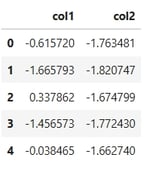
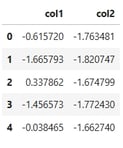
The sum of the explained variance ratio for the principal components is approximately 80%. This indicates that the first two components, col1 and col2, collectively capture nearly 80% of the dataset's variance. These components effectively summarize the majority of the information contained in the original features, making them a powerful tool for visualization and interpretation.

Next, I will examine the PCA components (the transformed x and y axes) to understand how the original features contribute to these new dimensions and to identify any meaningful patterns or relationships in the data.

I am now comparing the PCA components (the new x and y axes) to the original dataset columns (the old x, y, and z axes). This comparison helps to interpret how the original features contribute to the principal components and provides insights into the relationships and patterns captured by PCA. By mapping the transformed data back to its original dimensions, I can better understand the underlying structure of the dataset and validate the effectiveness of the dimensionality reduction.

This analysis is fundamentally an eigenvalue problem, where the principal components are derived from the eigenvectors of the dataset's covariance matrix. By comparing the PCA components to the original dataset columns, we can interpret the principal components as follows:

First Principal Component (col1):
- Higher values along the col1 axis correspond to older customers.
- Lower values along the col1 axis indicate higher spending scores.
Second Principal Component (col2):
- Higher values along the col2 axis correspond to higher income levels.

This interpretation provides meaningful insights into how the original features (age, income, and spending score) influence the principal components, enabling a clearer understanding of the dataset's structure.

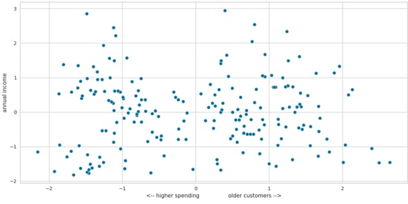
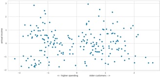
The PCA results suggest that the highest spenders are typically young or relatively young customers. Additionally, there appears to be no significant correlation between spending rate and income, which aligns with the findings from the earlier cluster analysis.

To further validate these conclusions, I will examine the correlation heatmap of the dataset before applying PCA. This will help determine whether similar relationships and patterns are evident in the original feature space.

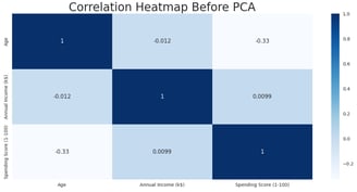
The correlation heatmap reveals the following key insights:

Annual Income shows almost no correlation with age or spending score.
There is a moderate negative correlation between customer age and spending score, indicating that younger customers tend to have higher spending scores, while older customers tend to spend less.

These findings are consistent with the conclusions drawn from the PCA results and the earlier cluster analysis, further validating the observed patterns in the dataset.

Code Availability

The complete code used for this analysis is available on my GitHub repository. You can access it at the following link:
https://github.com/pipe1223/deepFraud/tree/master/Mall_segment

Feel free to explore, reuse, or provide feedback on the implementation!