The Vision Transformer (ViT)

Understanding Vision Transformer Architecture

Let us take sometime now to understand the Vision Transformer Architecture. This is the link to the original vision transformer paper: https://arxiv.org/abs/2010.11929.

The Vision Transformer (ViT) is a type of Transformer architecture designed for image processing tasks. Unlike traditional Transformers that operate on sequences of word embeddings, ViT operates on sequences of image embeddings. In other words, it breaks down an input image into patches and treats them as a sequence of learnable embeddings.

At a broad level, what ViT does is, it:

1. Creates Patch Embeddings

2. Passes embeddings through Transformer Blocks

3. Performs Classification

Create Dataset and DataLoader

We can use PyTorch's ImageFolder DataSet library to create our Datasets. For ImageFolder to work this is how your data folder needs to be structured.

All the images of each class will be the train and test sub folders.

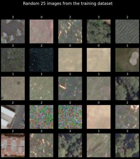
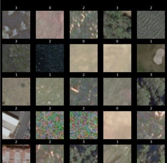
We can visualize a few training dataset images and see their labels

Create Patch Embedding Layer

For the ViT paper, we need to perform the following functions on the image before passing to the MultiHead Self Attention Transformer Layer

1. Convert the image into patches of 16 x 16 size.

2. Embed each patch into 768 dimensions. So each patch becomes a [1 x 768] Vector. There will be $N = H times W / P^2$ number of patches for each image. This results in an image that is of the shape [14 x 14 x 768]

3. Flatten the image along a single vector. This will give a [196 x 768] Matrix, which is our Image Embedding Sequence.

4. Prepend the Class Token Embeddings to the above output

5. Add the Position Embeddings to the Class Token and Image Embeddings.

Converting the image into patches of 16 x 16 and creating an embedding vector for each patch of size 768.

This can be accomplished by using a Conv2D Layer with a kernel_size equal to patch_size and a stride equal to patch_size. We can pass a random image into the convolutional layer and see what happens

Prepending the Class Token Embedding and Adding the Position Embeddings

Put the PatchEmbedddingLayer Together

We will inherit from the PyTorch nn.Module to create our custom layer which takes in an image and throws out the patch embeddings which consists of the Image Embeddings, Class Token Embeddings and the Position Embeddings.

Creating the Multi-Head Self Attention (MSA) Block.

As a first step of putting together our transformer block for the Vision Transformer model, we will be creating a MultiHead Self Attention Block.

Let us take a moment to understand the MSA Block. The MSA block itself consists of a LayerNorm layer and the Multi-Head Attention Layer. The layernorm layer essentially normalizes our patch embeddings data across the embeddings dimension. The Multi-Head Attention layer takes in the input data as 3 form of learnable vectors namely query, key and value, collectively known as qkv vectors. These vectors together form the relationship between each patch of the input sequence with every other patch in the same sequence (hence the name self-attention).

So, our input shape to the MSA Block will be the shape of our patch embeddings that we made using the PatchEmbeddingLayer -> [batch_size, sequence_length, embedding_dimensions]. And the output from the MSA layer will be of the same shape as the input.

Creating the Machine Learning Perceptron (MLP) Block

The Machine Learning Perceptron (MLP) Block in the transformer is a combination of a Fully Connected Layer (also called as a Linear Layer or a Dense Layer) and a non-linear layer. In the case of ViT, the non-linear layer is a GeLU layer. The transformer also implements a Dropout layer to reduce overfitting. So the MLP Block will look something like this:

Input → Linear → GeLU → Dropout → Linear → Dropout

According to the paper, the first Linear Layer scales the embedding dimensions to the 3072 dimensions (for the ViT-16/Base). The Dropout is set to 0.1 and the second Linear Layer scales down the dimensions back to the embedding dimensions.

The Transformer Block

Creating the ViT Model

Finally, let’s put together our ViT Model. It’s going to be as simple as combining whatever we have done till now. One slight addition will be the classifier layer that we will add. In ViT the classifier layer is a simple Linear layer with Layer Normalization. The classification is performed on the zeroth index of the output of the transformer.

Train this model

Conclusion

This step-by-step guide has helped you(me) understand the Vision Transformer.

PS. This my note so no discussion here

PS. The real reason that we have no discussion here because I don't want to maintain the forum.